|
Here I convolve an input signal, f, with a system impulse response, g, and plot the results, y = f*g, at each step of the computation. This GIF shows the processes involved in computing the discrete convolution. The steps are flip, slide, and sum. The impulse response, g, is flipped about the origin then a discrete sum is calculated at each incremental shift to obtain the updated output convolution. 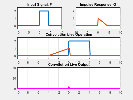 As you watch the video, note the following...
1. The convolution is the product of the overlapping areas as the signal is shifted. 2. The output signal peaks when both signals overlap completely. 3. The original signals both have non-zero values between 0 and 4 units. The output has non-zero values between 0 and 8 units.
2 Comments
Snell's Law of Refraction... I made these visualizations of Snell's Law using MATLAB. More details to follow (hopefully soon)! 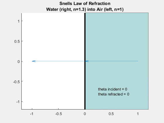 Figure 2: A ray shown refracting between a change in media from water into air. The ray is totally reflected when the incident wave has reached the critical angle. 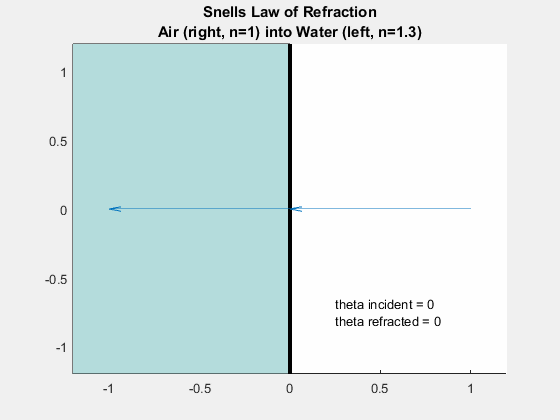 Figure 2: A ray shown refracting between a change in media from air into water. Note, the ray never totally reflects because the refractive index of air is less than that of water.
Below are my notes taken from MIT 8.02x Electricity and Magnetism (with experiments) taught by Dr. Walter Lewin back in the early 2000's.
Playlist: https://www.youtube.com/playlist?list=PLyQSN7X0ro2314mKyUiOILaOC2hk6Pc3j
Lecture 1: Coulomb's Law, Electric Charges and Forces
Lecture 2: Electric Field Lines, Superposition, Inductive Charging, Induced Dipoles Lecture 3: Electrostatics, Electric Flux, Gauss's Law Lecture 4: Electrostatic Potential, Equipotential Surfaces Lecture 5: E = - Grad(V), Conductors, Electrostatic Shielding Lecture 6: High voltage breakdown, lightning, sparks, St. Elmo's fire Lecture 7: Capacitance, Electric Field Energy Lecture 8: Polarization, Dielectrics, Van de Graaff Generator, Capacitors [*] Lecture 9: Electric Currents, Resistivity, Conductivity, Ohm's Law Lecture 10: Batteries, Kirchoff's Rule, Circuits Lecture 11: Magnetic Fields, Lorentz Force, Electric Motors Lecture 12: Exam 1 Review Lecture 13: Moving charges in B-fields, Cyclotrons Lecture 14: Biot-Savart, Div(B)=0, High-Voltage Power Lines Lecture 15: Ampere's Law, Solenoids Lecture 16: Electromagnetic Induction, Faraday's Law, Lenz's Law Lecture 17: Motional EMF, Dynamos, Eddy Currents, Magnetic Braking Lecture 18: Displacement Current, Synchronous Motors Lecture 19: Magnetic LEvitation, Superconductivity, Aurora Borealis Lecture 20: Inductance, RL Circuits, Magnetic Field Energy Lecture 21: Magnetism... Diamagnetism, Paramagnetism, Ferromagnetism Lecture 22: Magnetism... Magnetic field effect on materials, historicis Lecture 23: Exam 2 Review Lecture 24: RC Circuits and Transformers Lecture 25: Driven LRC circuits, metal detectors Lecture 26: Travelling waves, standing waves, musical instruments Lecture 27: Destructive Resonance, Electromagnetic Waves, Speed of Light Lecture 28: Poynting Vector, Oscillating Charges, Polarization, Radiation Pressure Lecture 29: Snell's Law, Index of Refraction, Huygen's Principle Lecture 30: Polarizers, Malus' Law, Light Scattering, Blue Skies Lecture 31: Rainbows, Halos, Sun Dogs Lecture 32: Exam 3 Review Lecture 33: Double-Slit Interference, Interferometers Lecture 34: Diffraction Gratings, Angular Resolution Lecture 35: Doppler Effect, Big Bang, Cosmology Lecture 36: Last Lecture
Click READ MORE to see lecture notes ----------------------------------->
A couple of years back I went through the MIT Open Courseware videos from Dr. Arthur Mattuck's Spring 2003 Differential Equations course. I watched the videos in the morning while eating breakfast and would re-derive the results from the video when I got to school. Unfortunately, I did not keep very detailed notes. I have found myself going back to the videos to refresh my knowledge on certain subjects, but I can't always remember which video contains which topic. For future reference I will start keeping track of keywords for each video and putting them below.
Playlist: https://www.youtube.com/playlist?list=PLEC88901EBADDD980
Lecture 1: First order ODEs of the form y' = f(x,y)
Lecture 2: Numerical solutions to differential equations by Euler's Method Lecture 3: First-order linear equations and the separation of variables Lecture 4: Change of variables and substitutions Lecture 5: Autonomous differential equations, integral curves, critical points Lecture 6: Complex numbers, polar form Lecture 7: Linear first order ODEs
Click READ MORE to continue reading ------------->
Here are my notes from Gilbert Strang's MIT Open Courseware Class in Linear Algebra. Here is a link to the YouTube playlist of all lectures. Lecture 1: Column and Row Space Visualization of Matrix [Really awesome lecture]
Lecture 2: Elimination, Back-Substitution, Elimination Matrices, Matrix Multiplication Lecture 3: Matrix Multiplication, Matrix Inversion, Gauss-Jordan Lecture 4: Inverse of AB, Product of Elimination Matrices, A=LU Lecture 5: PA=LU, Vector Spaces and Subspaces Lecture 6: Vector Spaces and Subspaces Lecture 7: Algorithm for Finding the Nullspace [Ax=0] Lecture 8: Complete Solution of Ax=b Lecture 9: Linear Independence, Spanning a Space, Basis, Dimension Lecture 10: The Four Fundamental Subspaces Lecture 11: Bases of Vector Spaces, Rank 1 Matrices Lecture 12: Graphs and Networks Lecture 13: Review Practice Problems Lecture 14: Orthogonal Vectors and Subspaces Lecture 15: Projection, Least Squares, Projection Matrix Lecture 16: Projection Matrices, Least Squared continued Lecture 17: Orthogonal Basis, Gram-Schmidt, Orthogonal Matrix Lecture 18: Determinants 1/2 Lecture 19: Determinants 2/2, Cofactor Expansion Lecture 20: Matrix Inversion and Determinants [Great Lecture, Lost Notes...] Lecture 21: Introduction to Eigenvalues and Eigenvectors Lecture 22: Matrix Diagonalization [S-1 * A * S = L], Powers of A, Fibonacci Example [*] Lecture 23: Application of Linear Algebra to Differential Equations Lecture 24: Markov Matrices and Fourier Series Lecture 24b: Review and Practice Problems Lecture 25: Symmetric Matrices Facts Lecture 26: Complex Vectors and Matrices, Fourier Matrix, FFT [Matrix Factorization] Lecture 27: Positive Definite Matrices Lecture 28: Positive Definite Matrices, Similar Matrices Lecture 29: Singular Value Decomposition [SVD] Lecture 30: Linear Transformations Lecture 31: Change of Basis, Image Compression Lecture 32: Review and Practice Problems Lecture 33: Inverses, Course Review Lecture 34: Review I have been covering the topic of plane waves quite a bit recently. After my post on the "phase circle" I got to thinking about wave polarization. In this post I will describe the polarization of plane waves. For now, I am going to upload a few simple videos, then I will come back to provide detail in a bit. Initial DetailsThe examples shown below display the x-component (red), y-component (yellow), and total field (purple) of a time varying signal of the form: F = A*cos(wt - Bz + phi) Where we are fixed at a location in space (say, z=0). If we decompose F into x and y, we have F = A*cos(wt + phi_x)*x_hat + A*cos(wt + phi_y)*y_hat where the amplitude, A, is a complex number. Now we can enforce a difference in phase between the x and y component of our field. It is this difference in phase between our components that gives us a sense of polarization. If phi_x equals phi_y then the wave is said to be linearly polarized. If phi_x equals phi_y +- 90 degrees then the wave is circularly polarized. Otherwise, in the most general case, the sum of the components trace out an ellipse as a function of time, called elliptical polarization. Linear Polarization Circular Polarization Elliptical Polarization
This morning as I was browsing the internet i came across this neat graphic. Every point is moving back and forth along a single axis in a sinusoid manner. This person incrementally adds more points to the plot and keeps track of the path of motion in a very colorful way!
I saw the graphic below a few years back. It is much simpler but illustrates the same sinsusoidal motion along a fixed direction where each point is offset in phase from its neighbor rendering the interesting rotation effect we see.
My Implementation
I couldn't resist putting together my own implementation. Below is a gif I created and the code I used to generate it. The sinusoidal variation along an axis is relatively straightforward, the only part that requires much thought is the initial phase offset. If you don't get that right, things get weird, but they also get very cool!
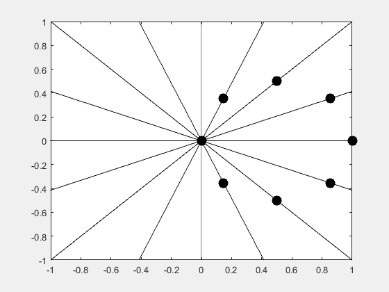
What's Actually Happening?
To understand what's actually happening, try focusing on one single point. Notice that it only moves back and forth along a single line, it does not rotate around the page. The rotation effect is a result of all the points moving at once. I can tell a point to move back and forth along a line using the standard equation for a line, y = mx + b, or I can decompose my line into x- and y-directed components. I chose to define unit vectors x and y that together always point me in the correct direction but whose amplitude I can vary sinusoidally. Look back at that point from before. Notice as the point gets closer to the edge of the frame it appears to slow down and as it moves to the center it speeds up. Using trigonometry, the amplitude varies like:
A = cos(theta) and theta takes on values between 0 and 2*pi so that A varies from -1 to 1. The amplitude at each point varies in this same way, but I include another argument in my sinusoid to offset each point in phase. A = cos(theta + phi) where phi is called the phase offset and allows me to start each point at a different initial position along the axis of motion. MATLAB Code
% Simple code to plot a phase circle
deltapi = pi/8; theta = 0 : deltapi : pi-deltapi; x = cos(theta); % x-directed vector y = sin(theta); % y-directed vector fig1 = figure(1); for angle = 0: pi/64 : 2*pi A = cos(angle+theta); % Amplitude scaling factor with phase offset figure(1); plot(A.*x, A.*y, 'ok', 'MarkerSize', 10, 'MarkerFaceColor','k'); hold on; % Plot straight line paths for i=1:length(theta) plot(2*[-cos(theta(i)) +cos(theta(i))], 2*[-sin(theta(i)) +sin(theta(i))],'color','k'); end hold off; xlim([-1 1]); ylim([-1 1]); drawnow; % pause(.15); end The Euclidean Algorithm is a method for calculating the greatest common divisor of 2 integers. It was Euclid, who in 300 BC, first presented the idea in his famous work entitle "The Elements." This technique is fascinating mathematically but also has many widespread applications. In fact, it is the GCD that makes secure public communication (via public key encryption) possible! A couple of years back I was going through Dr. Albert Meyer's MIT 6.042J (Math for CS) lectures where the importance of this very old algorithm was impressed upon me. It was here that I first learned of the Extended Euclidean Algorithm for calculating the Greatest Common Divisor. I will present the XGCD but let's first look at the plain old GCD. GCD - Euclidean MethodLet's begin with a recursive form of the greatest common divisor. We iterate through this procedure until the y value is zero, our final solution is in the x place. GCD( x, y ) = GCD( y, rem(x,y) ) What is interesting is that each iteration of the GCD is exactly equal to its predecessor. For instance, let's trace our way through a simple example. GCD(72, 26) = GCD(26, 20) = GCD(20, 6) = GCD(6, 2) = GCD(2,0) = 2 To emphasize what I mean, think about this... GCD(72,26) = GCD(6,2) If you don't see it at first, try plugging it into a calculator. This is a very important detail that emphasizes the strength of the procedure.
XGCD - PulverizerThe Extended Euclidean Algorithm (Bezout's Identity) not only calculates the GCD as is done using the general Euclidean Algorithm but also computes coefficients at each step such that we can express the current terms (a and b) of the GCD as a linear combination of the original inputs, x and y. That is, given 2 inputs x and y, we want to calculate GCD(x,y). At each step we calculate GCD(a_i, b_i). The first few iterations look like this.... GCD(x,y) = GCD(a_1, b_1) = GCD(a_2, b_2) = ..... where of course a_i = b_i-1. At each step we can find scalars c,d,e,f such that a_i = cx + dy b_i = ex + fy. In the initial step we can clearly represent x and y as x = a_0 = 1*x + 0*y [c = 1, d = 0] y = b_0 = 0*x + 1*y [e = 0, f = 1] If you haven't already, check out my example in the attached PDF, also shown below. I step through the XGCD algorithm to find the GCD of 899 and 493. MATLAB Code is attached here. Because at each iteration i, we have a_i = b_i-1, from the step GCD(a,b) = GCD(b, a%b), it follows naturally that c_i = e_i-1 and d_i = f_i-1. Where again c and d are coefficients that allow us to reconstruct our inputs x and y at any given iteration such that a_i = c*x + d*y and y_i = e*x + f*y. It is only slightly more complicated to calculate coefficients e and f, but for now I'll just present them below for completeness. e_i = c_i-1 - q_i-1*e_i-1 and f_i = d_i-1 - q_i-1*f_i-1 XGCD Example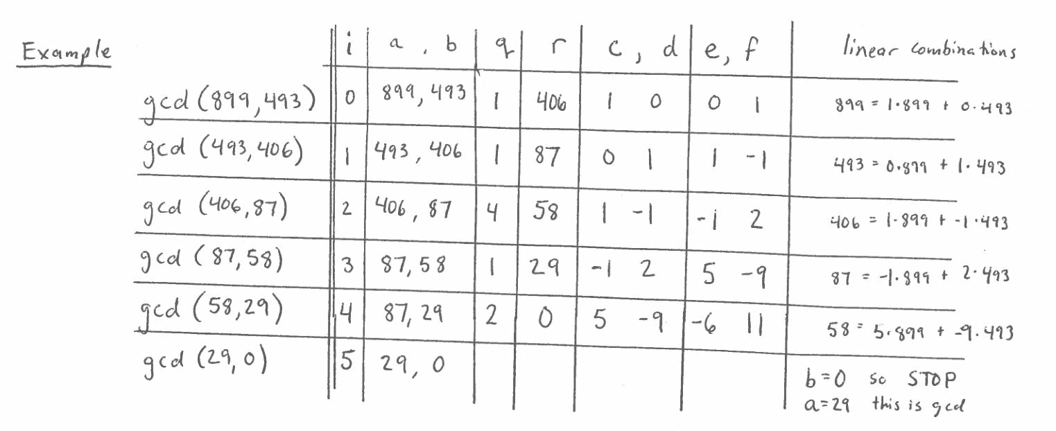 This example calculates the greatest common divisor of 899 and 493. At each step of the algorithm you will see
i, the iteration number, a and b, the current inputs to gcd, q, the quotient, where q = floor(a/b), r, the remainder, where r = a - q*b, c and d, coefficients such that a_i = cx + dy, e and f , coefficients such that b_i = ex + fy. Note that c, d, e, and f are set to 1, 0, 0, and 1 on the first iteration to show that x = a_0 = 1*x + 0*y [c = 1, d = 0] y = b_0 = 0*x + 1*y [e = 0, f = 1] and the subsequent values of the coefficient are calculated using the above expressions. In this post I will begin to explain the notion of Period and Wavelength as it is found in the plane wave solution to a second-order homogeneous wave equation. I will start with a general solution to a source-free wave equation and introduce the notion of phase velocity which will help clarify the relationship between the temporal period (period), spatial period (wavelength), and the properties of our propagation region. I will expand upon these concepts by implementing a form of the analytical solution in Matlab. The real part of our solution takes the form: F = A cos(wt - Bx + p). Where..... w (omega) is the angular velocity, and w = 2*pi*f, B (Beta) is the phase constant, and B = 2*pi/L, p (theta) is the phase offset, f is frequency and f=1/T, L (lambda) is wavelength. With this in mind we can re-write our solution using more familiar terms. F = A cos( t/T*2*pi - x/L*2*pi + p ) The argument of the above sinusoid is the phase term. To find the phase velocity we take a time derivative of the phase term and solve for the time rate of change of position. The time derivative of the phase gives us the instantaneous frequency, but, here we assume plane wave propagation where the phase is constant, thus the derivative is zero. The time rate of change of position produces a term we call the phase velocity. d/dt(phase) = 2*pi/T + 2*pi/L*[d/dt(x)] = 0 Vp = d/dt(x) = L/T We now have an important relation between the frequency and wavelength. Vp = f*L = w/B The phase velocity is determined by the properties of the media we are located in, that is, the permeability (mu) and pemittivity (epsilon). Vp = 1/sqrt(mu * epsilon) Our phase velocity is determined by our space, the time variation (frequency/period) is generally set by our source. In some sense, this means the "wavelength" or spatial period of our signal is set by these other two parameters and is more of a result than a chosen quantity. B = w/Vp For this reason, I chose to adopt the below form of my solution F = A cos(wt - w*z/Vp + p) which strictly enforces a spatial dependence on the frequency of our signal and the propagation velocity defined by our space of interest. This is likely over-complicated as most people are satisfied seeing B*z where I have removed the phase constant and replaced it with B=w/Vp. Maybe someone will find this helpful. By the way, the above equation is a general solution to the source-free wave equation c*c*d2/dx2(U) - d2/dt2(U) = 0. Computer Analytical SolutionI have implemented the above sinusoidal solution in Matlab to see how the field varies in both time and in space. More interesting and complicated examples are shown as well. #1 Simple Attenuating SinusoidMy first solution is propagating in free-space with a transmission frequency of 1 MHz and attenuation constant of 1e-3... F = A*exp(ax) * cos(wt - Bx + p) 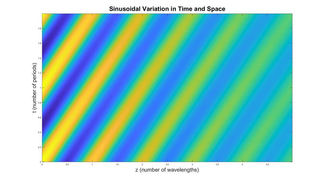 Figure 1. This figure shows the field magnitude as a function of wavelength (x-axis) and period (y-axis). A Horizontal slice of this image would show the field value as a function of wavelengths away from zero at a fixed instant in time. A vertical slice of this figure would give you the field values with respect to time at a single point in space. The following figures further illustrate this concept. 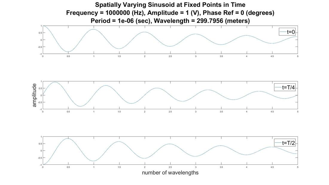 Figure 2. This figure shows 3 snapshots in time (at time 0, T/4, and T/2) throughout all of our space (5 wavelengths). These are 3 horizontal slices from Figure 1. 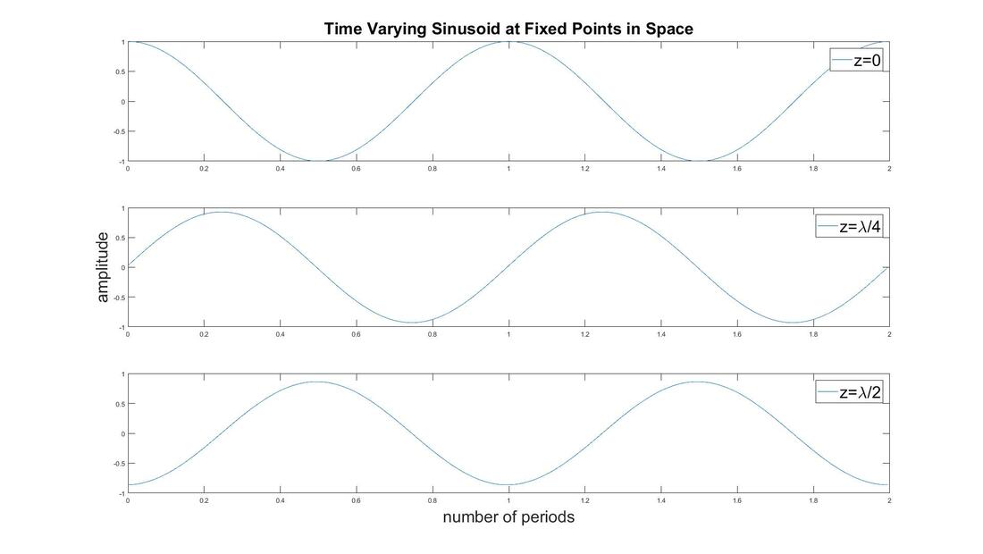 Figure 3. This figure shows the field values in time at 3 locations in space. These are 3 vertical slices from Figure 1. 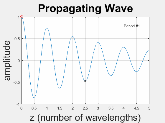 Figure 4. This video shows the field values in all of our space as a function of time. This essentially amounts to playing each horizontal slice from Figure 1 in succession. #2 Modulated SignalIn this section I modulate our carrier signal with a constant modulation frequency. 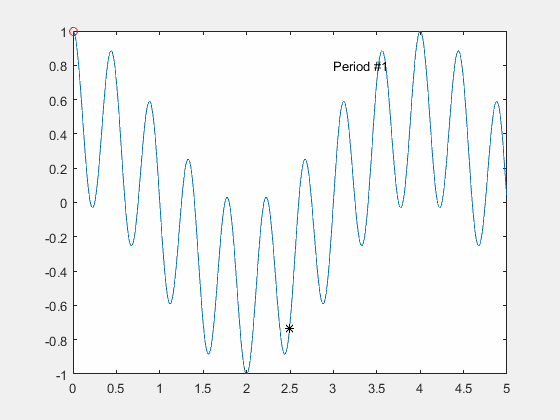 #3 Beat Wave GenerationIn this section I produce a beat wave as the product of 2 signals with differing frequencies. F = A cos(w0*t - Bx) + A cos(w1*t - Bx) 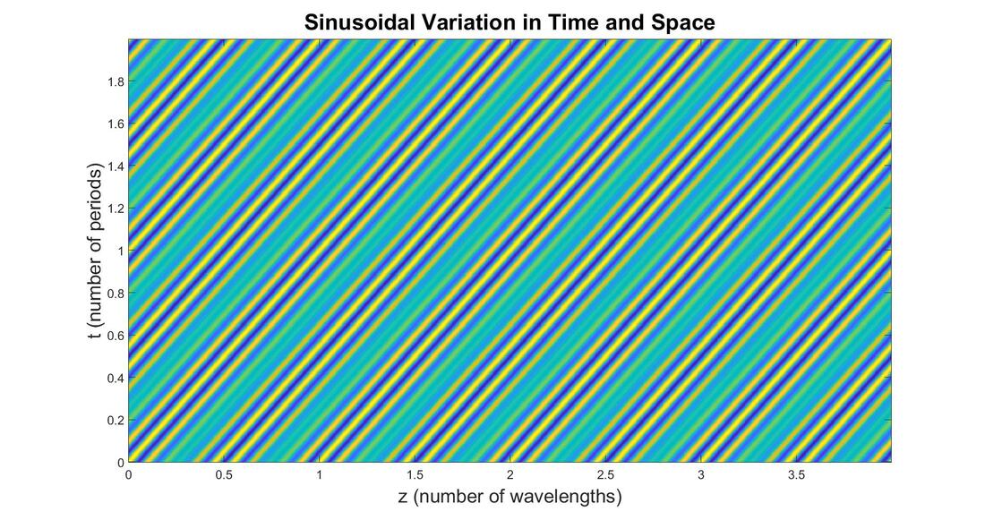 Figure 6. This figure shows the field magnitude as a function of wavelength (x-axis) and period (y-axis). A Horizontal slice of this image would show the field value as a function of wavelengths away from zero at a fixed instant in time. A vertical slice of this figure would give you the field values with respect to time at a single point in space. The following figures further illustrate this concept. 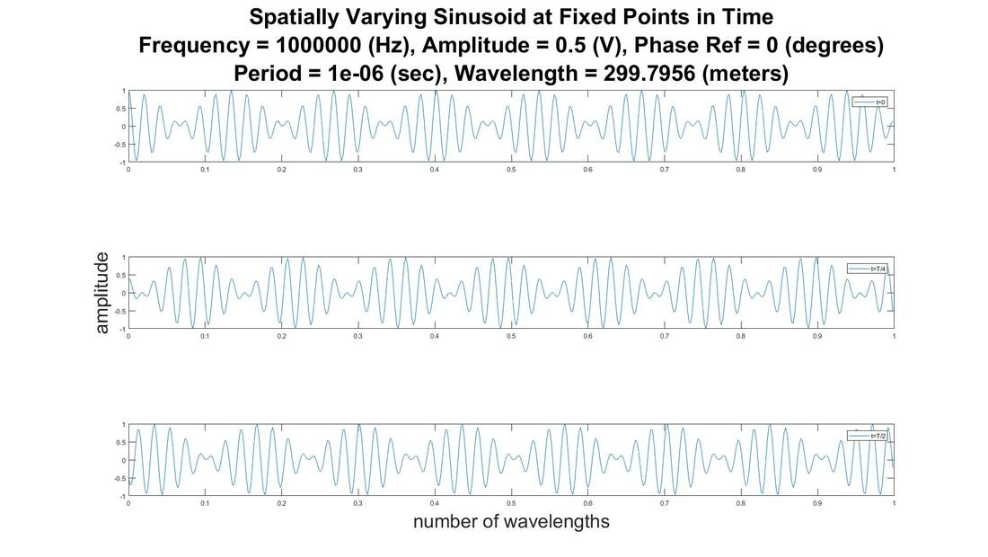 Figure 7. This figure shows 3 snapshots in time (at time 0, T/4, and T/2) throughout all of our space (5 wavelengths). These are 3 horizontal slices from Figure 6. 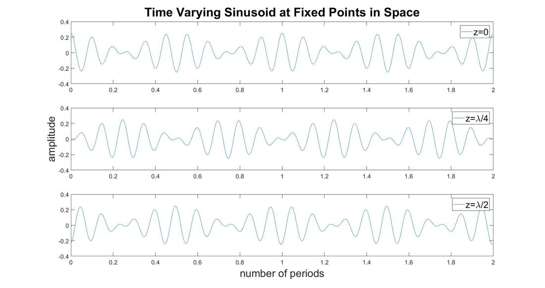 Figure 8. This figure shows the field values in time at 3 locations in space. These are 3 vertical slices from Figure 1. 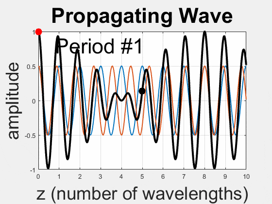 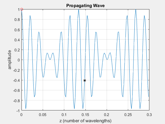 Figure 9. These videos show the field values in all of our space as a function of time. This essentially amounts to playing each horizontal slice from Figure 1 in succession. The first video shows the two separate sinusoids that are summed to create the beat wave.
|
AcademicsHere I will share material relating to my work in the classroom, both as a student and instructor. Archives
July 2020
Categories |
 RSS Feed
